1235 Maximum Profit in Job Scheduling - Hard

Problem:

We have n jobs, where every job is scheduled to be done from startTime[i] to endTime[i], obtaining a profit of profit[i].

You're given the startTime, endTime and profit arrays, return the maximum profit you can take such that there are no two jobs in the subset with overlapping time range.

If you choose a job that ends at time X you will be able to start another job that starts at time X.

Example 1:

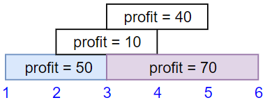
Input: startTime = [1,2,3,3], endTime = [3,4,5,6], profit = [50,10,40,70] Output: 120 Explanation: The subset chosen is the first and fourth job. Time range [1-3]+[3-6] , we get profit of 120 = 50 + 70.

Example 2:

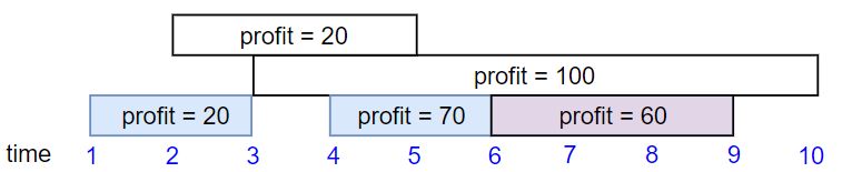
Input: startTime = [1,2,3,4,6], endTime = [3,5,10,6,9], profit = [20,20,100,70,60] Output: 150 Explanation: The subset chosen is the first, fourth and fifth job. Profit obtained 150 = 20 + 70 + 60.

Example 3:

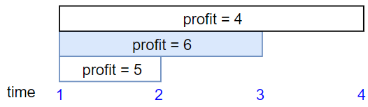
Input: startTime = [1,1,1], endTime = [2,3,4], profit = [5,6,4] Output: 6

Constraints:

• 1 <= startTime.length == endTime.length == profit.length <= 5 * 104
• 1 <= startTime[i] < endTime[i] <= 109
• 1 <= profit[i] <= 104

Problem Analysis:

High-Level Strategy:

The high-level strategy of this solution is to efficiently find the maximum profit that can be obtained by scheduling non-overlapping jobs. The algorithm sorts the jobs based on their end times, then uses dynamic programming to iteratively calculate the maximum profit at each step. It employs a bottom-up approach, where the dynamic programming table (dp) is filled iteratively, considering two options for each job: including the current job or excluding it. The key insight is to use binary search to efficiently find the closest non-conflicting job before the current one, which optimizes the overall time complexity.

Complexity Analysis:

1. Time Complexity:

   • Sorting the jobs based on end times takes O(n log n), where n is the number of jobs.
   • The dynamic programming loop iterates through each job once, and for each job, it performs a binary search, taking O(log n) time.
   • Overall, the time complexity is dominated by the sorting and is O(n log n).

2. Space Complexity:

   • The space complexity is primarily determined by the dynamic programming table (dp), which has a size of O(n + 1).
   • The additional space used for sorting the jobs is O(n) due to the zipped list.
   • The overall space complexity is O(n).

Solutions:

class Solution:
    def jobScheduling(self, startTime: List[int], endTime: List[int], profit: List[int]) -> int:
        # sort jobs based on endTime
        jobs = sorted(zip(startTime, endTime, profit), key=lambda x: x[1])
        number_of_jobs = len(profit)
      
        # init dp table where n is no of jobs to store max profit up to the no of jobs
        dp = [0] * (number_of_jobs + 1)
        
        for i, (current_start_time, current_end_time, current_profit) in enumerate(jobs):
            # Binary Search to find the closest non-conflicting job before current jon
            index = bisect_right(jobs, current_start_time, hi=i, key=lambda x: x[1])
            
            # To maximize profit, consider two options:
            #   a. The maximum profit without considering the current job (dp[i])
            #   b. The maximum profit considering the current job, plus the maximum profit
            #      from jobs that don't conflict with the current job (dp[index] + current_profit)
            # Take the maximum of these two options and update the dp array at index+1.
            dp[i + 1] = max(dp[i], dp[index] + current_profit)

        return dp[number_of_jobs]

Similar Questions